There are no items in your cart
Add More
Add More
| Item Details | Price | ||
|---|---|---|---|

Vector stores represent the foundational infrastructure powering the next generation of AI applications, transforming how machines understand, retrieve, and generate contextually relevant information.
Vector stores are specialized databases engineered to efficiently store, index, and retrieve highdimensional vector embeddings that encode semantic meaning from unstructured data. Unlike traditional databases that rely on exact keyword matching and structured queries, vector stores enable semantic similarity search by representing data as numerical vectors in multidimensional space.
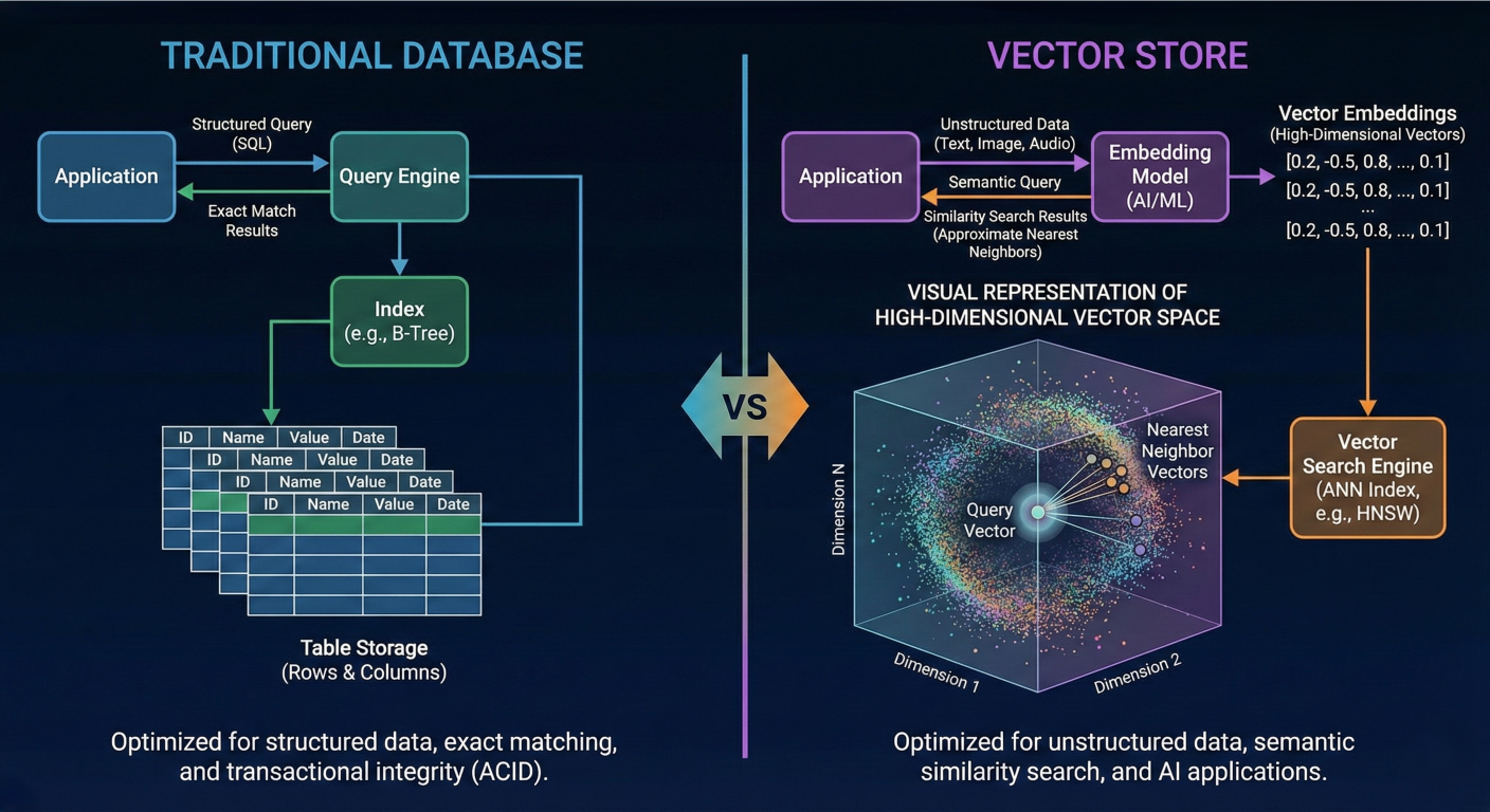
Architecture diagram showing traditional database vs vector store comparison with visual representation of high-dimensional vector space
When text, images, audio, or other data types are processed by machine learning models, they are transformed into vector embeddings—dense numerical arrays that capture the semantic essence of the original content. These embeddings typically range from 256 to 1536 dimensions for modern models like OpenAI's text-embedding-3-large, with each dimension representing learned features that encode meaning and relationships.
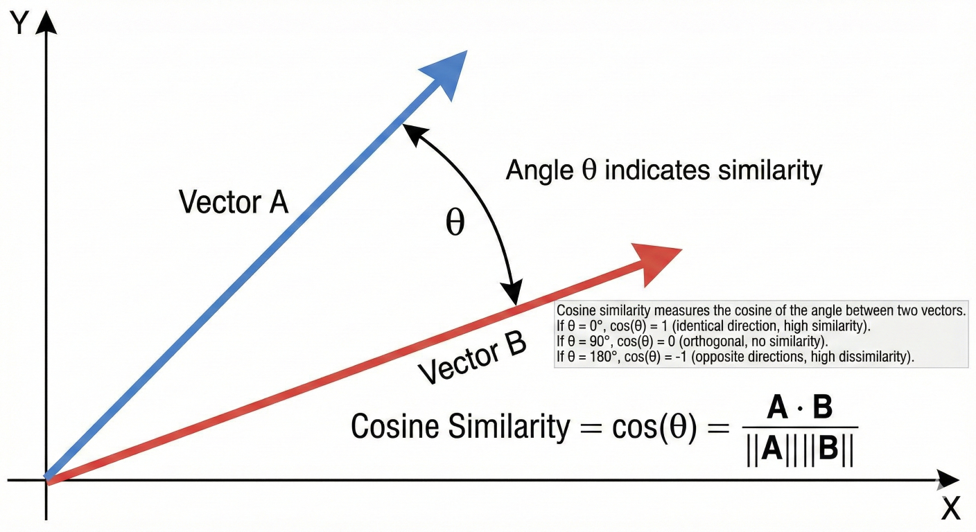
Vector embeddings operate on the principle that semantically similar content produces similar vector representations in high-dimensional space. This enables vector stores to perform similarity searches using mathematical distance metrics rather than lexical matching, fundamentally changing how information retrieval systems work.
The core mathematical relationship can be expressed through cosine similarity:
$ similarity = \frac{A \cdot B}{||A|| \times ||B||} = \cos(\theta) $
where A and B are vector embeddings, and θ represents the angle between them. Values closer to 1 indicate higher semantic similarity, while values approaching -1 suggest semantic opposition.
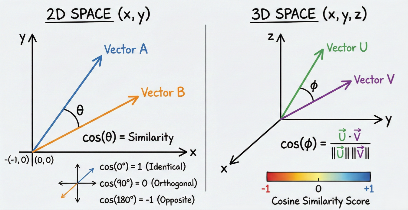
Visual diagram showing vector similarity calculation in 2D/3D space with cosine similarity representation
Retrieval-Augmented Generation represents a paradigm shift in how Large Language Models access and utilize external knowledge. RAG architecture consists of three fundamental components working in concert: the embedding model, vector store, and generative model.
Step 1: Knowledge Base Creation
The RAG pipeline begins with vectorization of external data sources. Documents, web pages, databases, or any text-based content are processed through embedding models to generate vector representations. These embeddings are then stored in the vector database alongside metadata and the original text chunks.
Step 2: Query Processing and Retrieval
When a user submits a query, the system transforms it into a vector embedding using the same embedding model used for the knowledge base. The vector store then performs similarity search to identify the most semantically relevant documents or passages.
Step 3: Context Augmentation
Retrieved relevant passages are combined with the user's original query to create an augmented prompt. This enriched context provides the LLM with specific, relevant information needed to generate accurate responses.
Step 4: Response Generation
The Large Language Model processes the augmented prompt, leveraging both its pre-trained knowledge and the retrieved contextual information to generate informed, factually grounded responses.
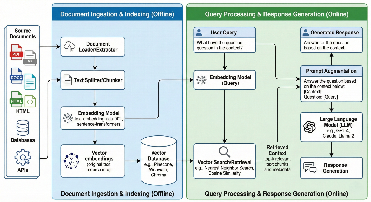
Detailed RAG architecture flowchart showing data flow from document ingestion through response generation
The vector store serves as the intelligent memory system for RAG applications. Unlike traditional databases that require exact matches, vector stores enable semantic retrieval where conceptually related information can be found even when using different terminology.
For example, a query about "machine learning algorithms" can retrieve documents discussing "artificial intelligence techniques," "neural networks," or "deep learning models" because their vector representations cluster in similar regions of the high-dimensional space
HNSW represents one of the most sophisticated and widely adopted graph-based indexing algorithms for approximate nearest neighbor search. The algorithm constructs a multi-layered graph structure that enables logarithmic search complexity while maintaining high accuracy.
The HNSW algorithm organizes vectors into hierarchical layers, where each layer contains a subset of the dataset with decreasing density as you move up the hierarchy. The bottom layer (Layer 0) contains all vectors and maintains the highest connectivity, while upper layers contain exponentially fewer nodes but enable rapid navigation across large distances in the vector space.
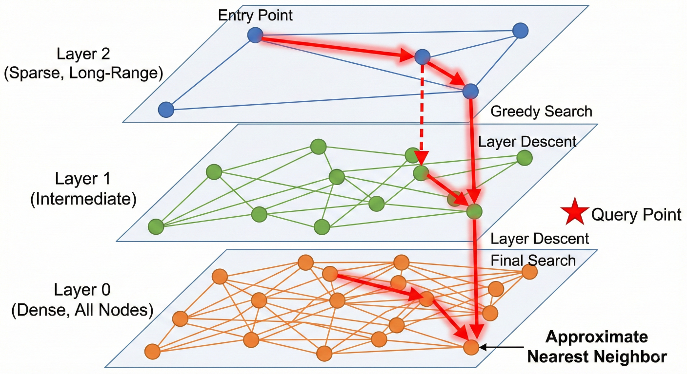
Multi-layer HNSW graph visualization showing hierarchical structure and search path traversal
1. Entry Point Selection: New vectors are assigned to layers probabilistically, with higher layers having lower probability
2. Graph Construction: Each vector establishes bidirectional connections with its nearest neighbors within each layer
3. Dynamic Updates: The algorithm supports real-time insertions and deletions without requiring complete index rebuilds
HNSW search follows a greedy traversal strategy across layers:
1. Entry Phase: Search begins at the highest layer from a single entry point
2. Layer Traversal: The algorithm navigates to the closest neighbors in the current layer
3. Layer Descent: Upon reaching a local minimum, search moves to the next lower layer
4. Final Retrieval: The process continues until reaching Layer 0, where the final k-nearest neighbors are identified
Performance Characteristics:
IVF-PQ combines clustering-based indexing with vector compression to achieve both speed and memory efficiency. This hybrid approach excels in scenarios requiring massive scale with controlled memory footprint.
The IVF component partitions the vector space into Voronoi cells using k-means clustering. Each cell represents a region of semantically similar vectors, dramatically reducing search scope during query time.
1. Clustering Phase: K-means algorithm partitions vectors into nlist clusters
2. Centroid Storage: Cluster centroids serve as coarse quantizers
3. Index Creation: Inverted lists map each centroid to vectors within its Voronoi cell
4. Search Execution: Queries are matched against centroids to identify relevant cells for detailed search
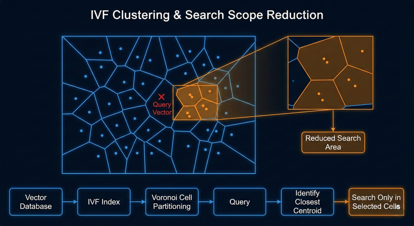
IVF clustering visualization showing Voronoi cells and search scope reduction
Product Quantization addresses memory constraints by compressing high-dimensional vectors while preserving similarity relationships. The technique splits vectors into sub-vectors and quantizes each sub-vector independently.
1. Vector Decomposition: D-dimensional vectors are split into m sub-vectors of dimension D/m
2. Codebook Generation: Each sub-vector space is quantized using k-means clustering
3. Encoding: Original vectors are replaced with codebook indices, reducing storage from 32bit floats to 8-bit codes
4. Distance Calculation: Similarity computations use pre-calculated lookup tables for efficient processing
Cosine similarity measures the angle between vectors, making it ideal for semantic similarity tasks where magnitude is less important than direction. This metric excels in natural language processing applications where document length shouldn't affect similarity scores.
Mathematical formulation:
cosine_similarity(A, B) = \frac{\sum_{i=1}^{n} A_i B_i}{\sqrt{\sum_{i=1}^{n} A_i^2} \times \sqrt{\sum_{i=1}^{n} B_i^2}}
Cosine Distance (used in vector databases) is calculated as:
cosine_distance = 1 - cosine_similarity
Advantages:
Geometric visualization of cosine similarity showing angle measurement between vectors
Euclidean distance measures the straight-line distance between vectors in high-dimensional space. This metric works well when both magnitude and direction matter for similarity determination.
Mathematical formulation:
euclidean_distance(A, B) = \sqrt{\sum_{i=1}^{n} (A_i - B_i)^2}
Use Cases:
Dot product similarity combines both direction and magnitude information while offering computational efficiency. For normalized vectors, dot product becomes equivalent to cosine similarity.
Mathematical formulation:
dot_product(A, B) = \sum_{i=1}^{n} A_i \times B_i
# Configure OpenAI API
import os
from langchain_community.embeddings import OpenAIEmbeddings
from langchain_community.vectorstores import Chroma
from langchain.docstore.document import Document

os.environ["OPENAI_API_KEY"] = "your-openai-api-key"

# Prepare sample documents
documents = [
    Document(
        page_content="Vector stores enable semantic search by storing high-dimensional embeddings.",
        metadata={"source": "tutorial", "category": "fundamentals"}
    ),
    Document(
        page_content="HNSW algorithm creates multi-layered graphs for efficient similarity search.",
        metadata={"source": "research", "category": "algorithms"}
    ),
    Document(
        page_content="RAG combines retrieval from vector stores with generative language models.",
        metadata={"source": "architecture", "category": "applications"}
    )
]

# Initialize embedding model
embeddings = OpenAIEmbeddings(
    model="text-embedding-3-small",
    dimensions=1536
)

# Create persistent vector store
vector_store = Chroma.from_documents(
    documents=documents,
    embedding=embeddings,
    collection_name="ai_knowledge_base",
    persist_directory="./chroma_storage"
)

# Perform similarity search with metadata filtering
query = "How does vector similarity search work?"
results = vector_store.similarity_search(
    query,
    k=2,
    filter={"category": "algorithms"}
)

# Display results with scores
for i, doc in enumerate(results):
    print(f"Result {i+1}: {doc.page_content}")
    print(f"Metadata: {doc.metadata}")
    print("-" * 50)
from langchain.chains import RetrievalQA
from langchain_openai import ChatOpenAI
from langchain.prompts import PromptTemplate

# Initialize GPT-4 for generation
llm = ChatOpenAI(
    model="gpt-4-turbo-preview",
    temperature=0.1,
    max_tokens=800
)

# Create custom RAG prompt template
rag_template = """
Use the following context to answer the question comprehensively.
If the context doesn't contain sufficient information, acknowledge this limitation.

Context: {context}

Question: {question}

Detailed Answer:"""

PROMPT = PromptTemplate(
    template=rag_template,
    input_variables=["context", "question"]
)

# Build RAG chain
qa_chain = RetrievalQA.from_chain_type(
    llm=llm,
    chain_type="stuff",
    retriever=vector_store.as_retriever(
        search_type="similarity_score_threshold",
        search_kwargs={
            "k": 4,
            "score_threshold": 0.7
        }
    ),
    chain_type_kwargs={"prompt": PROMPT},
    return_source_documents=True
)

# Execute RAG query
question = "What are the performance characteristics of HNSW algorithm?"
response = qa_chain({"query": question})

print(f"Question: {question}")
print(f"Answer: {response['result']}")
print(f"Sources used: {len(response['source_documents'])}")
import numpy as np
from sklearn.metrics.pairwise import cosine_similarity
from typing import List, Dict, Tuple
import uuid

class CustomVectorStore:
    """Production-ready vector store with advanced features"""

    def __init__(self, embedding_dimension: int = 1536):
        self.embedding_dim = embedding_dimension
        self.vectors = []
        self.documents = []
        self.metadata = []
        self.ids = []
        self.index_built = False

    def add_documents(self,
                     texts: List[str],
                     embeddings: List[List[float]],
                     metadatas: List[Dict] = None) -> List[str]:
        """Add documents with pre-computed embeddings"""

        doc_ids = [str(uuid.uuid4()) for _ in texts]

        if metadatas is None:
            metadatas = [{}] * len(texts)

        # Validate embedding dimensions
        for emb in embeddings:
            if len(emb) != self.embedding_dim:
                raise ValueError(f"Embedding dimension mismatch: {len(emb)} != {self.embedding_dim}")

        # Store data
        self.vectors.extend([np.array(emb, dtype=np.float32) for emb in embeddings])
        self.documents.extend(texts)
        self.metadata.extend(metadatas)
        self.ids.extend(doc_ids)

        self.index_built = False  # Invalidate index
        return doc_ids

    def build_index(self):
        """Build optimized index for fast similarity search"""
        if self.vectors:
            self.vector_matrix = np.vstack(self.vectors)
            # Normalize vectors for cosine similarity
            norms = np.linalg.norm(self.vector_matrix, axis=1, keepdims=True)
            self.normalized_vectors = self.vector_matrix / np.maximum(norms, 1e-8)
            self.index_built = True

    def similarity_search(self,
                         query_embedding: List[float],
                         k: int = 5,
                         filter_metadata: Dict = None,
                         similarity_threshold: float = 0.0) -> List[Dict]:
        """Advanced similarity search with filtering and thresholding"""

        if not self.vectors:
            return []

        if not self.index_built:
            self.build_index()

        # Normalize query vector
        query_vector = np.array(query_embedding, dtype=np.float32)
        query_norm = np.linalg.norm(query_vector)
        if query_norm > 0:
            query_vector = query_vector / query_norm

        # Calculate cosine similarities
        similarities = np.dot(self.normalized_vectors, query_vector)

        # Apply metadata filtering
        valid_indices = list(range(len(self.documents)))
        if filter_metadata:
            valid_indices = [
                i for i in valid_indices
                if all(self.metadata[i].get(k) == v for k, v in filter_metadata.items())
            ]

        # Apply similarity threshold
        valid_indices = [
            i for i in valid_indices
            if similarities[i] >= similarity_threshold
        ]
        # Get top-k results
        scored_indices = [(i, similarities[i]) for i in valid_indices]
        scored_indices.sort(key=lambda x: x[1], reverse=True)
        top_results = scored_indices[:k]

        # Format results
        results = []
        for idx, score in top_results:
            results.append({
                'id': self.ids[idx],
                'document': self.documents[idx],
                'metadata': self.metadata[idx],
                'similarity_score': float(score)
            })

        return results

    def get_statistics(self) -> Dict:
        """Return comprehensive vector store statistics"""
        if not self.vectors:
            return {"error": "No vectors stored"}

        similarities = cosine_similarity(self.vector_matrix)
        np.fill_diagonal(similarities, 0)  # Remove self-similarities

        return {
            "total_documents": len(self.documents),
            "embedding_dimensions": self.embedding_dim,
            "average_similarity": float(np.mean(similarities)),
            "similarity_std": float(np.std(similarities)),
            "memory_usage_mb": (self.vector_matrix.nbytes / 1024 / 1024),
            "unique_metadata_keys": list(set(
                key for meta in self.metadata for key in meta.keys()
            ))
        }

# Demonstration usage
custom_store = CustomVectorStore(embedding_dimension=1536)

# Sample embeddings (normally from actual embedding model)
sample_embeddings = [
    np.random.normal(0, 1, 1536).tolist() for _ in range(3)
]

sample_texts = [
    "Vector databases store high-dimensional embeddings for AI applications",
    "HNSW provides efficient approximate nearest neighbor search capabilities",
    "Product quantization reduces memory requirements for large-scale vector storage"
]

# Add documents to custom store
doc_ids = custom_store.add_documents(
    texts=sample_texts,
    embeddings=sample_embeddings,
    metadatas=[
        {"type": "definition", "complexity": "basic"},
        {"type": "algorithm", "complexity": "advanced"},
        {"type": "optimization", "complexity": "intermediate"}
    ]
)

# Perform similarity search
query_embedding = np.random.normal(0, 1, 1536).tolist()
search_results = custom_store.similarity_search(
    query_embedding=query_embedding,
    k=2,
    filter_metadata={"complexity": "advanced"},
    similarity_threshold=0.1
)

print("Custom Vector Store Search Results:")
for result in search_results:
    print(f"Score: {result['similarity_score']:.4f}")
    print(f"Document: {result['document'][:100]}...")
    print(f"Metadata: {result['metadata']}")
    print("-" * 60)
from llama_index.core import VectorStoreIndex, SimpleDirectoryReader
from llama_index.core import Settings
from llama_index.embeddings.openai import OpenAIEmbedding
from llama_index.core.documents import Document

# Configure LlamaIndex settings
Settings.embed_model = OpenAIEmbedding(
    model="text-embedding-3-large",
    dimensions=3072
)

# Create document collection
documents = [
    Document(
        text="Vector stores are fundamental infrastructure for modern AI applications, enabling semantic search and retrieval-augmented generation.",
        metadata={"category": "fundamentals", "difficulty": "beginner"}
    ),
    Document(
        text="HNSW algorithm constructs hierarchical navigable small world graphs that provide logarithmic search complexity for high-dimensional vector spaces.",
        metadata={"category": "algorithms", "difficulty": "advanced"}
    ),
    Document(
        text="RAG architecture combines vector retrieval with language model generation to produce factually grounded, contextually relevant responses.",
        metadata={"category": "architecture", "difficulty": "intermediate"}
    )
]

# Build vector index
index = VectorStoreIndex.from_documents(
    documents,
    show_progress=True
)

# Create query engine with advanced settings
query_engine = index.as_query_engine(
    similarity_top_k=3,
    response_mode="tree_summarize",
    verbose=True
)

# Execute complex query
complex_query = "Explain how HNSW algorithm enables efficient vector search in RAG systems"
response = query_engine.query(complex_query)

print(f"Query: {complex_query}")
print(f"Response: {response}")
print(f"Source nodes: {len(response.source_nodes)}")
Pinecone offers a fully managed, serverless vector database optimized for production AI applications. The platform abstracts infrastructure complexity while providing enterprise-grade performance and reliability.
Key Advantages:
Optimal Use Cases:
Pricing Considerations:
Weaviate combines vector search with graph database capabilities, enabling hybrid queries that seamlessly blend semantic similarity with structured data filtering. The platform excels in multi-modal applications involving text, images, and metadata.
Distinctive Features:
Optimal Use Cases:
Deployment Flexibility:
Milvus represents the gold standard for large-scale, distributed vector databases. Built for cloud-native environments, Milvus separates compute, storage, and metadata management for unlimited horizontal scaling.
Architectural Strengths:
Performance Characteristics:
Enterprise Deployment:
Chroma focuses on developer experience and AI application simplicity. Designed specifically for LLM applications, Chroma provides intuitive APIs and seamless integration with popular AI frameworks.
Developer-Centric Features:
Deployment Options:
pgvector extends PostgreSQL with native vector similarity search capabilities, enabling organizations to add vector search to existing relational database infrastructure.
Integration Benefits:
Performance Considerations:
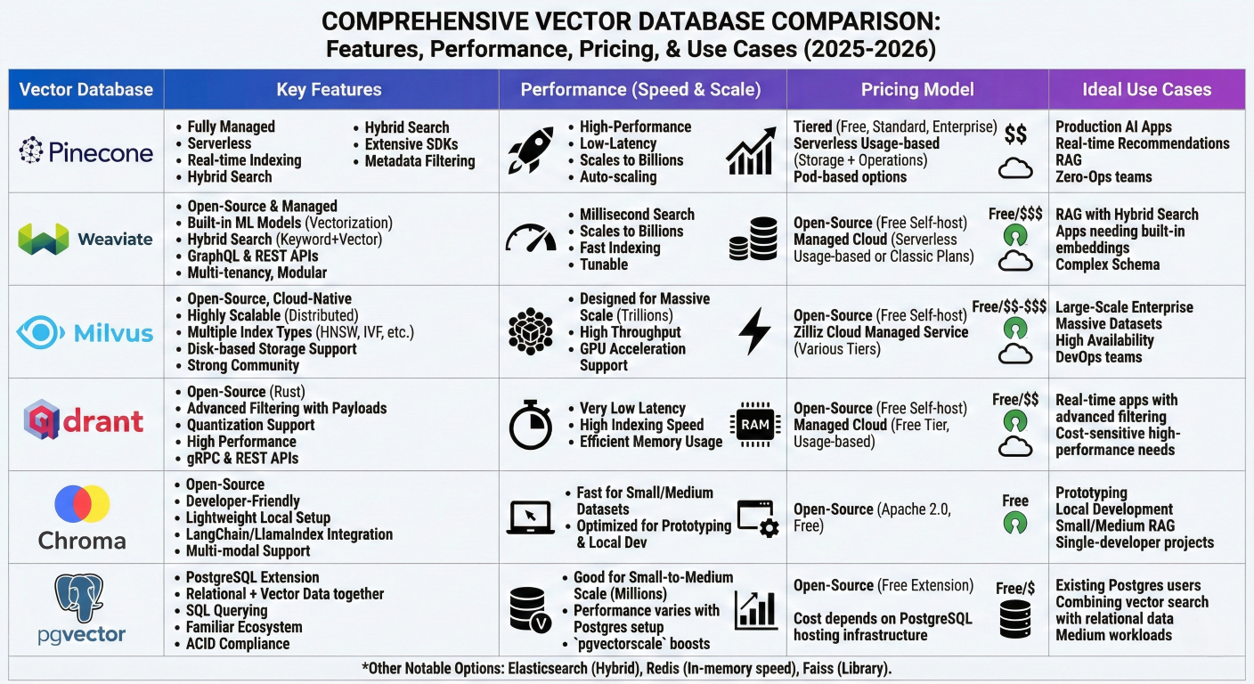
Comprehensive comparison table showing features, performance, pricing, and use cases across all major vector databases
| Database |
Deployment |
Best For | Scalability | Complexity | CostModel |
| Pinecone | Cloud-only |
Real-time apps, startups | Auto-scaling | Low | Usage-based |
| Weaviate | Hybrid | Multi-modal, hybrid search | Manual scaling | Medium | Open core |
| Milvus | Milvus | Enterprise, massive scale | Distributed | High | Open source |
| Chroma | Local/Cloud | Development, prototyping | Limited | Low | Open source |
| pgvector | Self-hosted E | Existing PostgreSQL users | PostgreSQL limits | Medium | Open source |
Real-time data synchronization represents one of the most critical challenges in production vector database deployments. Unlike traditional databases where updates are straightforward, vector stores must regenerate embeddings and update complex index structures.
Modern vector databases implement multi-tier freshness architectures to balance consistency with performance:
1. Hot Layer: Recently updated vectors stored in fast, queryable cache
2. Index Layer: Bulk of data in optimized, read-heavy indexes
3. Reconciliation Process: Background jobs merge hot layer into main indexes
4. Query Router: Intelligent routing across layers during search operations
Implementation Strategy:
class FreshnessAwareVectorStore:
    def __init__(self):
        self.main_index = {}  # Stable, optimized index
        self.fresh_cache = {}  # Recent updates
        self.pending_updates = []  # Batch processing queue

    def add_document(self, doc_id, embedding, metadata):
        # Add to fresh cache for immediate availability
        self.fresh_cache[doc_id] = {
            'embedding': embedding,
            'metadata': metadata,
            'timestamp': time.time()
        }

        # Queue for batch index update
        self.pending_updates.append(doc_id)

        # Trigger batch processing if threshold reached
        if len(self.pending_updates) > 1000:
            self.batch_update_index()

    def search(self, query_embedding, k=10):
        # Search both main index and fresh cache
        main_results = self.search_main_index(query_embedding, k)
        fresh_results = self.search_fresh_cache(query_embedding, k)

        # Merge and re-rank results
        return self.merge_results(main_results, fresh_results, k)
Distributed vector databases must address unique challenges in partitioning high-dimensional data while maintaining search accuracy.
Sharding Approaches:
1. Hash-Based Sharding: Distribute vectors using hash functions for even distribution
2. Locality-Sensitive Sharding: Group similar vectors on same nodes to improve search accuracy
3. Hybrid Sharding: Combine hash distribution with locality preservation
4. Dynamic Re-sharding: Automatic rebalancing based on query patterns and data growth
Performance Optimization Techniques:
Memory efficiency becomes critical as vector datasets grow to billions of vectors:
Tiered Storage Strategy:
Embedding model changes can invalidate entire vector indexes, requiring careful migration strategies:
Version Management Approach:
Lorem Ipsum is simply dummy text of the printing and typesetting industry. Lorem Ipsum has been the industry's standard dummy text ever since the 1500s, when an unknown printer took a galley of type and scrambled it to make a type specimen book.
Vector quality validation ensures embedding integrity and search accuracy:
Quality Metrics:
The vector database market is experiencing unprecedented growth, with market size projected to reach $10.6 billion by 2032 from $2.2 billion in 2024, representing a 21.9% compound annual growth rate. This explosive growth is driven by the widespread adoption of generative AI, RAG architectures, and semantic search applications.
Enterprise AI Adoption:
Technology Convergence:
Next-generation indexing techniques are addressing current limitations in accuracy, speed, and memory efficiency:
SPANN (Spiked Product Quantization with Approximate Nearest Neighbor):
Neural Information Retrieval:
Specialized hardware is emerging to accelerate vector operations:
Vector Processing Units (VPUs):
Extended context windows in LLMs (up to 1M+ tokens) are changing vector database requirements:
Implications for Vector Stores:
AI agents are driving new requirements for vector databases:
For Enterprises Planning Production Deployment:
Stay Current with Industry Evolution:
The future of AI applications fundamentally depends on efficient vector storage and retrieval systems. By mastering these technologies today, developers and organizations position themselves at the forefront of the AI revolution, ready to build the next generation of intelligent, context-aware applications that will define the digital landscape of tomorrow.
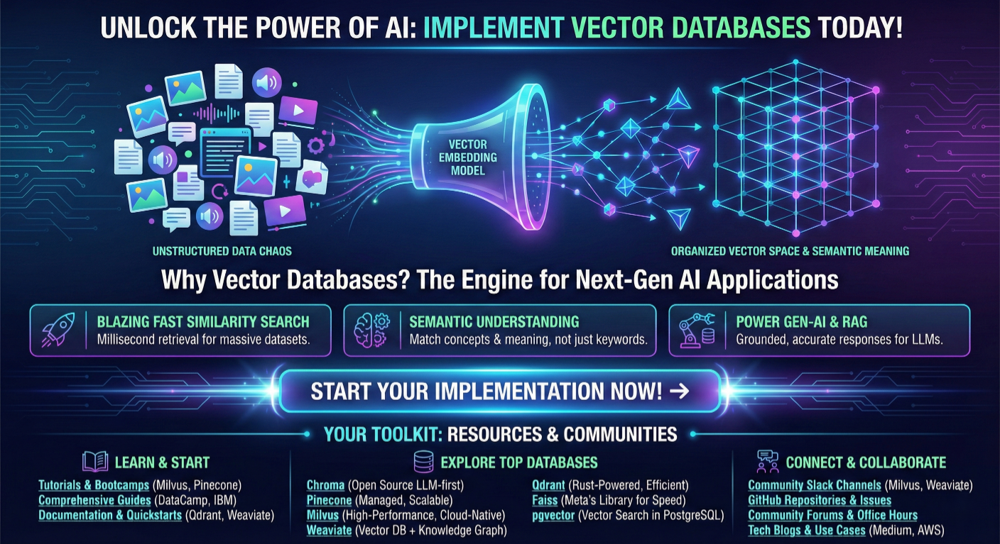
Call-to-action graphic encouraging readers to implement vector databases with links to resources and communities
Ready to implement vector stores in your AI applications? Start with our code examples above, join the community discussions, and begin building the future of intelligent search and retrieval systems today.

{{AUTHOR}}
 Launch your Graphy