RAG in Generative AI: The Definitive 2025 Masterclass

Introduction: The RAG Revolution in 2025

If you have been following the trajectory of Generative AI, you know that the initial euphoria of 2023—where we marveled that ChatGPT could write a poem—has settled into the pragmatic engineering reality of 2025. We are no longer asking if Large Language Models (LLMs) are useful; we are asking how to make them accurate, reliable, and deeply knowledgeable about proprietary data. The answer, resoundingly, is Retrieval-Augmented Generation (RAG).

RAG has graduated from a clever "hack" to the central architectural pillar of enterprise AI. It addresses the fundamental "parametric memory" limitation of LLMs. A model like GPT-4o or Claude 3.5 Sonnet is essentially a frozen snapshot of the internet at a specific point in time. It knows everything about the Battle of Hastings but nothing about the Q4 sales report you generated this morning. It can write Python code, but it cannot cite your company's internal security compliance standards.

RAG bridges this gap by dynamically injecting relevant context into the model's inference window, grounding its creative power in your specific, verifiable facts. It transforms the LLM from a "Know-It-All" into a "Know-Where-To-Look" engine.

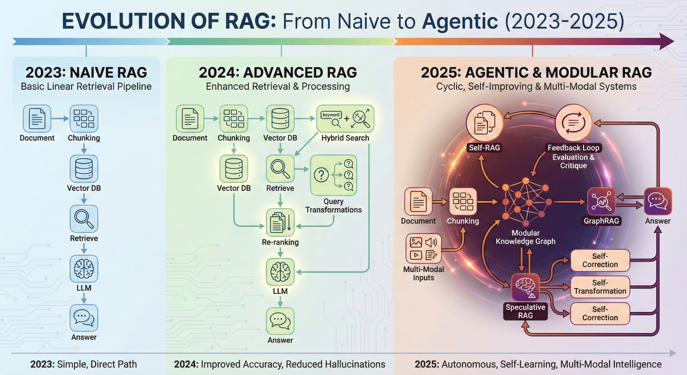
Detailed description about picture/Architecture/Diagram: A comprehensive timeline and evolutionary diagram of RAG. The left side shows "2023: Naive RAG" with a simple linear path (Document -> Chunk -> Vector DB -> Retrieve -> LLM). The center shows "2024: Advanced RAG" introducing Re-ranking, Query Transformations, and Hybrid Search. The right side shows "2025: Agentic & Modular RAG" featuring a cyclic graph with Feedback Loops, Self-Correction, Knowledge Graphs, and Multi-Modal inputs, labeled with terms like "Self-RAG," "GraphRAG," and "Speculative RAG." 

The Case for RAG: Why Not Just Fine-Tune?

A persistent question in the developer community remains: "Why shouldn't I just fine-tune the model on my data?" It is an intuitive thought—if the model learns from data, teaching it my data should work, right? In 2025, the industry consensus is heavily weighted toward RAG for knowledge retrieval, reserving fine-tuning for behavioral adaptation.

To understand this, we must look at the mechanics of how models store information. Fine-tuning adjusts the weights of the neural network. It "bakes" information into the model's fuzzy parametric memory. RAG, conversely, provides an "open-book" exam setting where the model has access to the source text.

The hybrid approach is often the gold standard: use Fine-Tuning to teach the model how to speak (e.g., "Act as a senior legal analyst"), and use RAG to tell it what to speak about (e.g., "Here is the contract from 2024").

The Evolution of RAG: From Naive to Agentic

We are currently witnessing the third generation of RAG architectures.

1. Naive RAG (2023): The "Hello World" of RAG. Split text, embed, retrieve top-k, generate. It suffers from low precision ("garbage in, garbage out") and low recall (missing relevant info).
2. Advanced RAG (2024): Introduced pre-retrieval optimization (query rewriting) and post-retrieval optimization (re-ranking, hybrid search). This improved accuracy significantly by treating retrieval as a multi-stage process.
3. Modular & Agentic RAG (2025): The current state-of-the-art. RAG is no longer a linear pipeline. It is a system of modules (Retrievers, Generators, Evaluators, Routers) that an AI Agent orchestrates. The agent can decide to search, verify the result, search again if the first attempt failed, or even use tools.

Part 1: The Core Architecture of Modern RAG

To build a robust RAG system, we must treat it as a data engineering challenge first and an AI challenge second. The quality of your retrieval is strictly capped by the quality of your data ingestion and indexing.

1.1 Ingestion and Parsing: The Foundation

Before vectors exist, we have documents. In the enterprise, these are rarely clean text files. They are PDFs with multi-column layouts, PowerPoints with embedded charts, and Excel sheets with critical financial data.

The "Garbage In, Garbage Out" Reality If your parser reads a PDF and merges a header from page 1 with a footer from page 2, your chunk will be nonsensical. Modern parsers like LlamaParse or Unstructured.io use vision-based models to "see" the document layout. They identify that a table is a table, not just a stream of text.

• Insight: For 2025, OCR (Optical Character Recognition) is not enough. You need Layout Analysis. If a table spans two pages, the parser must reconstruct it into a single semantic unit (e.g., Markdown table or JSON) before chunking. Otherwise, the row data loses its column headers, and the semantic meaning is destroyed.

1.2 Chunking Strategies: The Art of Segmentation

Chunking is the process of breaking large documents into smaller pieces that fit into the LLM's context window. It seems trivial, but it is one of the highest-leverage hyperparameters in RAG.

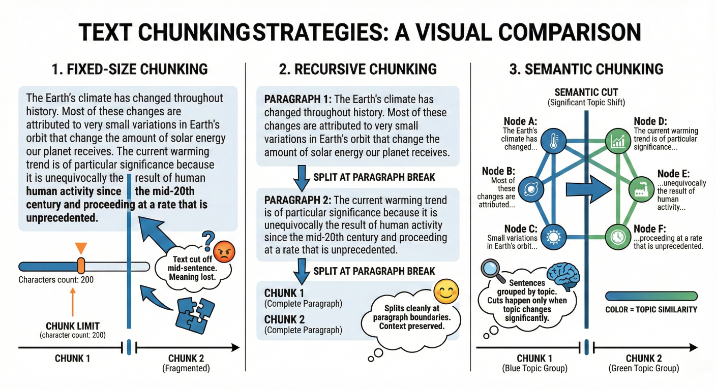
Fixed-Size Chunking

The simplest approach. You slice text every $N$ characters or tokens (e.g., 512 tokens) with an overlap (e.g., 50 tokens).

• Pros: Computationally cheap and easy to implement.
• Cons: It is semantically blind. It might cut a sentence in half, or worse, separate a question from its answer. This leads to "context fragmentation".

Recursive Character Chunking

The industry standard for generic text. It attempts to split hierarchically: first by paragraphs (\n\n), then by newlines (\n), then by sentences (.), and finally by words.

• Why it works: It tries to preserve the natural structure of the text, keeping related ideas together. It is the default in LangChain for good reason.

Semantic Chunking

A more advanced method for 2025. Instead of relying on punctuation, it uses an embedding model to measure the semantic similarity between sequential sentences.

1. Process: Calculate the cosine similarity between Sentence i and Sentence i+1.
2. Threshold: If the similarity score drops below a certain threshold (e.g., a sudden change in topic from "Revenue" to "HR Policies"), a cut is made.
3. Result: Chunks represent coherent topics rather than arbitrary lengths. Benchmarks show this significantly improves retrieval relevance because the vector is "purer".

Agentic / Propositional Chunking

This is the cutting edge. It uses an LLM to rewrite the text into atomic "propositions"—standalone statements of fact—before embedding.

• Original Text: "The iPhone 15, released in 2023, features a titanium frame."
• Propositions:
1. "The iPhone 15 was released in 2023."
2. "The iPhone 15 features a titanium frame."

• Benefit: If a user asks "What is the iPhone 15 made of?", the retrieval system matches Proposition 2 perfectly, without the noise of the release date. This minimizes the "distractor" information that can confuse vector similarity.

1.3 Indexing: The Vector Database Landscape

Once chunked, data is passed through an embedding model (like OpenAI's text-embedding-3 or open-source equivalents like bge-m3) to create vectors. These vectors are stored in a Vector Database (Vector DB).

HNSW vs. IVF: The Indexing Wars

When configuring a Vector DB (like Pinecone, Milvus, or Weaviate), you typically choose between two indexing algorithms: HNSW and IVF. Understanding the difference is critical for production performance.

HNSW (Hierarchical Navigable Small World)

• Mechanism: Imagine a multi-layered graph. The top layer is a sparse highway system; the bottom layer is the local streets. Searching starts at the top to get to the general neighborhood of the query vector, then drills down to the local streets for precision.
• Performance: It is the current gold standard for speed and recall (accuracy). It delivers sub-millisecond search times.
• Cost: It is memory-hungry. The graph structure must be held in RAM for speed. A dataset of 1 million vectors (dim=128) can consume ~1.6GB of RAM.

• Mechanism: It clusters the vector space into Voronoi cells (regions). When a query comes in, it identifies the closest cell and only searches vectors inside that cell.
• Performance: Slightly slower than HNSW and potentially lower recall if the correct answer lies just across the border of a cell (the "boundary problem").
• Cost: Much more memory efficient. It works well for massive datasets (100M+ vectors) where RAM is a constraint.
  

Comparison of Vector Indexing Algorithms

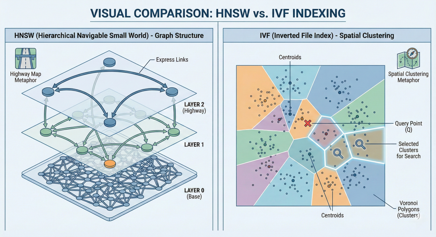
Detailed description about picture/Architecture/Diagram: Visual comparison of HNSW vs IVF. HNSW is depicted as a multi-layered graph structure with "express links" on top layers and dense connections on the bottom layer, resembling a highway map. IVF is depicted as a 2D space divided into Voronoi polygons (clusters) with a query point highlighting specific cells to search.

1.4 Retrieval: Beyond Dense Vector Search

In 2023, we relied on "Dense Retrieval"—matching the query vector to document vectors. In 2025, we know this is insufficient. Dense vectors capture semantic meaning ("dog" matches "canine"), but they often fail at exact keyword matching ("Error code 543" might not match "Issue 543" if the embedding model wasn't trained on those specific tokens).

Hybrid Search: The Industry Standard

Hybrid search combines two retrieval methods:

1. Dense Vector Search: Uses embeddings (Cosine Similarity). Good for concepts and natural language questions.
2. Sparse Keyword Search (BM25/Splade): Uses keyword frequency. Good for exact matches (names, SKUs, acronyms, specific error codes).

Where r(d) is the rank of document d in one of the retrieval lists (e.g., the vector list or the keyword list), and k is a constant (usually 60). This formula ensures that a document appearing in both lists gets a significantly higher score than a document appearing at the top of only one list.

Re-Ranking: The Quality Filter

Retrieving the top 100 documents is fast (milliseconds). But feeding 100 documents to an LLM is expensive and confusing. We need a filter. Enter the Cross-Encoder Re-ranker (e.g., Cohere Rerank, BGE-Reranker).

• Bi-Encoder (Standard): Encodes Query and Document separately. Fast but loses nuance.
• Cross-Encoder (Re-ranker): Feeds the Query and Document together into a BERT model. The model pays attention to the interaction between every word in the query and every word in the document.
• Workflow:
  1. Retrieve: Get top 100 candidates via Hybrid Search (Fast).
  2. Re-rank: Score those 100 using a Cross-Encoder (Slow but precise).
  3. Select: Take the top 5 re-ranked docs for the LLM context. This "Two-Stage Retrieval" pipeline is the standard for high-performance RAG in 2025, maximizing both speed and accuracy.

Part 2: Advanced RAG Techniques and Patterns

Once you have mastered the basics, you will encounter edge cases where simple RAG fails. This is where advanced patterns come into play.

2.1 Parent Document Retrieval (Small-to-Big)A fundamental tension in RAG is chunk size.

• Small chunks are better for retrieval because they are specific (high vector similarity).
• Large chunks are better for generation because they provide context (cohesion).

1. Split: Divide document into "Parent" chunks (e.g., 2000 tokens) and "Child" chunks (e.g., 200 tokens).
2. Index: Embed and index only the Child chunks.
3. Retrieve: Search against Child chunks.
4. Fetch: When a Child match is found, retrieve its Parent chunk to send to the LLM. This gives you the precision of small-chunk retrieval with the rich context of large-chunk generation.
   

2.3 GraphRAG: Structuring the Unstructured

One of the most significant advancements in 2025 is GraphRAG. Standard Vector RAG treats documents as a bag of isolated vectors. It struggles with "global" questions like * "How do the themes in Document A relate to the conclusions in Document B?"*

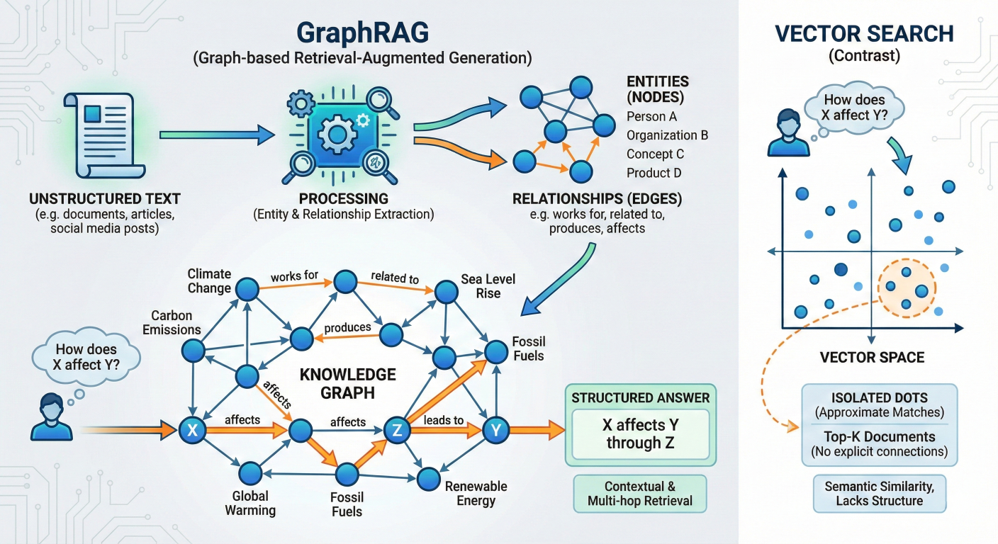
<--- Detailed description about picture/Architecture/Diagram: Diagram of GraphRAG. It shows unstructured text being processed into "Entities" (Nodes) and "Relationships" (Edges) to form a Knowledge Graph. A user query "How does X affect Y?" is shown traversing the edges of the graph to find the answer, contrasting with a Vector Search which just finds isolated dots in a 2D space. --->

GraphRAG combines Knowledge Graphs (KG) with LLMs.

• Ingestion: An LLM extracts entities (People, Places, Concepts) and relationships (Works_For, Located_In, Causes) from the text and builds a graph structure (e.g., in Neo4j).
• Retrieval: The system can perform graph traversals. It can "walk" from Entity A to Entity B to find hidden connections that no single document explicitly states.
• Performance: Benchmarks show GraphRAG recovering accuracy on schema-heavy queries (like supply chain tracing) where Vector RAG scores near zero. It adds explainability and structured reasoning to the pipeline.

When to use GraphRAG?

• Vector RAG: Good for "What does X say about Y?" (Local context).
• GraphRAG: Good for "How does X impact the entire system of Y?" (Global context).
  

2.4 RAPTOR (Recursive Abstractive Processing for Tree-Organized Retrieval)

RAPTOR is designed for long-context question answering where the answer spans multiple parts of a document.

• Concept: It clusters chunks based on semantic similarity and then summarizes those clusters. It then clusters the summaries and summarizes them again, building a hierarchical tree of information.
• Retrieval: When a query comes in, it can match against the high-level summaries (the "forest") to find the right section, and then drill down into the specific chunks (the "trees").
• Impact: This helps with "meta-questions" like "Summarize the financial performance of Q3," which requires synthesizing information from multiple pages.

Part 3: The Era of Agentic RAG

We are moving away from linear chains (Step A -> Step B -> Step C) toward Agentic Workflows (Loops, Conditionals, Decision Making).

3.1 Self-RAG (Self-Reflective RAG)

Self-RAG adds a "Critic" to the loop. It is a framework where the model learns to critique its own retrieval and generation. It introduces Reflection Tokens:

• Retrieve: The model decides if it needs to retrieve. If the user asks "Hi", it skips retrieval. If they ask "Explain the 2025 tax code", it triggers retrieval.
• IsRel (Is Relevant): After retrieving, the model grades the document. "Is this actually relevant to the query?"
• IsSup (Is Supported): After generating an answer, the model checks, "Is this sentence supported by the retrieved document?"
• IsUse (Is Useful): "Is this a helpful answer?"

3.2 Corrective RAG (CRAG)

CRAG focuses specifically on the quality of retrieved documents.

1. Retrieve: Fetch documents.
2. Evaluate: A lightweight evaluator model grades the documents as "Correct", "Ambiguous", or "Incorrect".
3. Action:

• Correct: Proceed to generation.
• Incorrect: Discard and trigger a fallback (e.g., search Google/Web).
• Ambiguous: Reformulate the query and try again. This ensures that the Generator LLM is never fed "poisoned" (irrelevant) context, which is the leading cause of bad answers.
  

3.3 Speculative RAG

This architecture optimizes for both speed and accuracy using a "Drafter-Verifier" approach.

1. Drafting: A smaller, faster model (e.g., Llama-3-8B) generates multiple "draft" answers in parallel, each based on a different subset of retrieved documents.
2. Verification: A larger, smarter model (e.g., GPT-4o) reviews the drafts. It acts as an Editor-in-Chief, selecting the best parts of each draft or synthesizing them into a final high-quality response.

• Benefit: It reduces latency (because drafts are fast) and reduces the "Lost-in-the-Middle" problem (because each draft focuses on a small subset of data).
  

3.4 MemoRAG (Memory-Augmented)

Standard RAG is stateless; it forgets the previous query instantly. MemoRAG introduces a global memory module.

• Concept: It compresses the dataset into a "global memory" (up to 1M tokens).
• Workflow: When a query comes in, the system first consults the global memory to get a "fuzzy" understanding or clues. It uses these clues to guide the precise retrieval.
• Use Case: Ideal for summarizing entire books or understanding long-term trends in data that span hundreds of documents.

Part 4: Technical Implementation Guide (Python)

Let's transition from theory to code. We will compare the two dominant frameworks: LangChain and LlamaIndex, and implement advanced features.

4.1 LangChain: The Composable Builder

LangChain is famous for its "Lego block" philosophy. In 2025, the standard way to write LangChain is using LCEL (LangChain Expression Language), a declarative way to pipe components together.

Code Example: A Modern LangChain RAG Pipeline with Hybrid Search and Re-ranking

Why Choose LlamaIndex? LlamaIndex excels at handling hierarchical data. It has native support for "Index Composition"—building an index of indices (e.g., a Summary Index for each document, and a Vector Index for the summaries). This is powerful for complex document sets.

4.3 Implementing Multi-Query Retrieval (LangChain)

To implement the Multi-Query pattern discussed earlier, we wrap the base retriever.

This simple addition effectively "automates" prompt engineering for the retrieval step, making the system robust against vague user inputs.

Part 5: Evaluation - Moving Beyond "Vibe Checking"

Key RAG Metrics

Ragas Implementation Code

This pipeline allows you to practice Test-Driven Development (TDD) for AI. If you change your chunk size from 500 to 1000, run the eval. If Context Precision drops, you know the larger chunks introduced too much noise. This data-driven approach is the only way to optimize systematically.

Part 6: Production Challenges & Optimization

Building a RAG demo in a notebook is easy. Deploying it to 10,000 users is a war zone. Here are the critical challenges and solutions for production RAG in 2025.

6.1 The Cost of RAGRAG is operationally expensive.

• Vector Storage: Hosting 10M vectors on a managed service like Pinecone or Weaviate costs hundreds of dollars a month.
• Inference: If you retrieve 10 chunks (2000 tokens) for every query, and use GPT-4, the costs accumulate rapidly.

Optimization Strategies:

6.2 Latency Kills

Users expect chat interfaces to be instant.

• The Bottleneck: The Re-ranker is often the slowest part, taking 500ms-1s.
• The Fix: Use ColBERT (Contextualized Late Interaction over BERT). It offers the accuracy of a cross-encoder with the speed of a bi-encoder by delaying the interaction step to the very end of the process.
• Streaming: Always stream the response. It does not make the generation faster, but it reduces the Time to First Token (TTFT). The user sees text appearing instantly, which psychologically masks the latency.

6.3 The "Lost in the Middle" Phenomenon

Research has shown that LLMs are biased towards information at the beginning and end of the context window. Information buried in the middle is often ignored.

• The Fix: LongContextReorder. When you retrieve 10 documents, do not just pass them in order 1-10. Re-order them so the most relevant documents are at position 1 and position 10, with the least relevant in the middle (e.g., ). LangChain has this utility built-in.

Conclusion: The Future is Hybrid

As we look toward the latter half of 2025 and into 2026, the line between "Model" and "Retrieval" is blurring. With the rise of "Long Context" models (like Gemini 1.5 Pro supporting 1M+ tokens), some argue RAG is dead—just paste the whole database into the prompt!

However, RAG is not dead; it is evolving. Even with a 1M token window, filling it is slow and expensive. RAG will remain the efficient "pre-filter" that selects the most relevant 1% of data to feed the model. Furthermore, Agentic RAG—where the model can actively browse, verify, and correct its own research—is unlocking capabilities we are only beginning to understand.

Call to Action: The theory is vast, but mastery comes from practice.

1. Start Small: Clone the LangChain or LlamaIndex repository.
2. Build: Implement the "Multi-Query" pipeline from Part 4.
3. Evaluate: Run the Ragas evaluation on your own data.