There are no items in your cart
Add More
Add More
| Item Details | Price | ||
|---|---|---|---|

We are currently living through a paradigm shift in software engineering. The rise of Large Language Models (LLMs) like GPT-4, Claude, and Llama has transformed how we interact with data. However, as powerful as these models are, they suffer from a critical limitation: they are frozen in time. A model trained in 2023 has no knowledge of the events of 2024. Furthermore, a model trained on the public internet has absolutely no insight into your private corporate data, your customer support logs, or your proprietary codebase.
For an intermediate developer or data scientist, this presents a frustrating paradox. You have the most powerful reasoning engine in history at your fingertips, but it is effectively amnesiac regarding the specific information you actually care about.
The industry's answer to this problem is Retrieval-Augmented Generation (RAG). Instead of retraining the model (which is prohibitively expensive) or fine-tuning it (which is complex and often degrades general reasoning capabilities), we simply provide the relevant information to the model at the exact moment it needs it.
But this solution creates a new engineering challenge. If you have a corpus of 10 million distinct documents, how do you find the exact three paragraphs that are relevant to a user's specific query? And how do you do it in less than 50 milliseconds so that the chat experience feels real-time?
Traditional keyword search (like SQL's LIKE operator or even BM25) fails here because it relies on exact word matches. If a user asks for "instructional guides for new employees," a keyword search might miss a document titled "Onboarding Handbook" because the words don't overlap.
This is where Vector Search and FAISS (Facebook AI Similarity Search) enter the picture. FAISS is the engine that powers the "long-term memory" of modern AI systems. It allows us to search by meaning rather than by keywords. It is the mathematical bridge that connects a user's intent to your vast repository of data.
In this extensive guide, we are going to tear apart the FAISS library. We will look under the hood at how it manages to search billions of vectors in milliseconds. We will explore the different index types—from the brute-force exactness of IndexFlatL2 to the graph-navigating speed of HNSW. We will write Python code to build our own semantic search engine, and we will discuss the production-grade optimizations required to run this at scale.
Whether you are building a simple chatbot or a massive enterprise knowledge management system, understanding FAISS is no longer optional—it is a fundamental skill for the Generative AI era.
To truly understand why we use FAISS, we must first situate it within the broader architecture of a Generative AI application. The Retrieval-Augmented Generation (RAG) pattern is the standard architecture for giving LLMs access to external data.
A RAG pipeline is essentially a mechanism for injecting context into an LLM's prompt. It consists of two distinct workflows: the Ingestion Loop (offline) and the Inference Loop (online/runtime).
This is where we prepare our "memory."
text-embedding-3 or an open-source model like all-MiniLM-L6-v2). This model converts the text into a fixed-size list of floating-point numbers—a vector.This is what happens when a user asks a question.
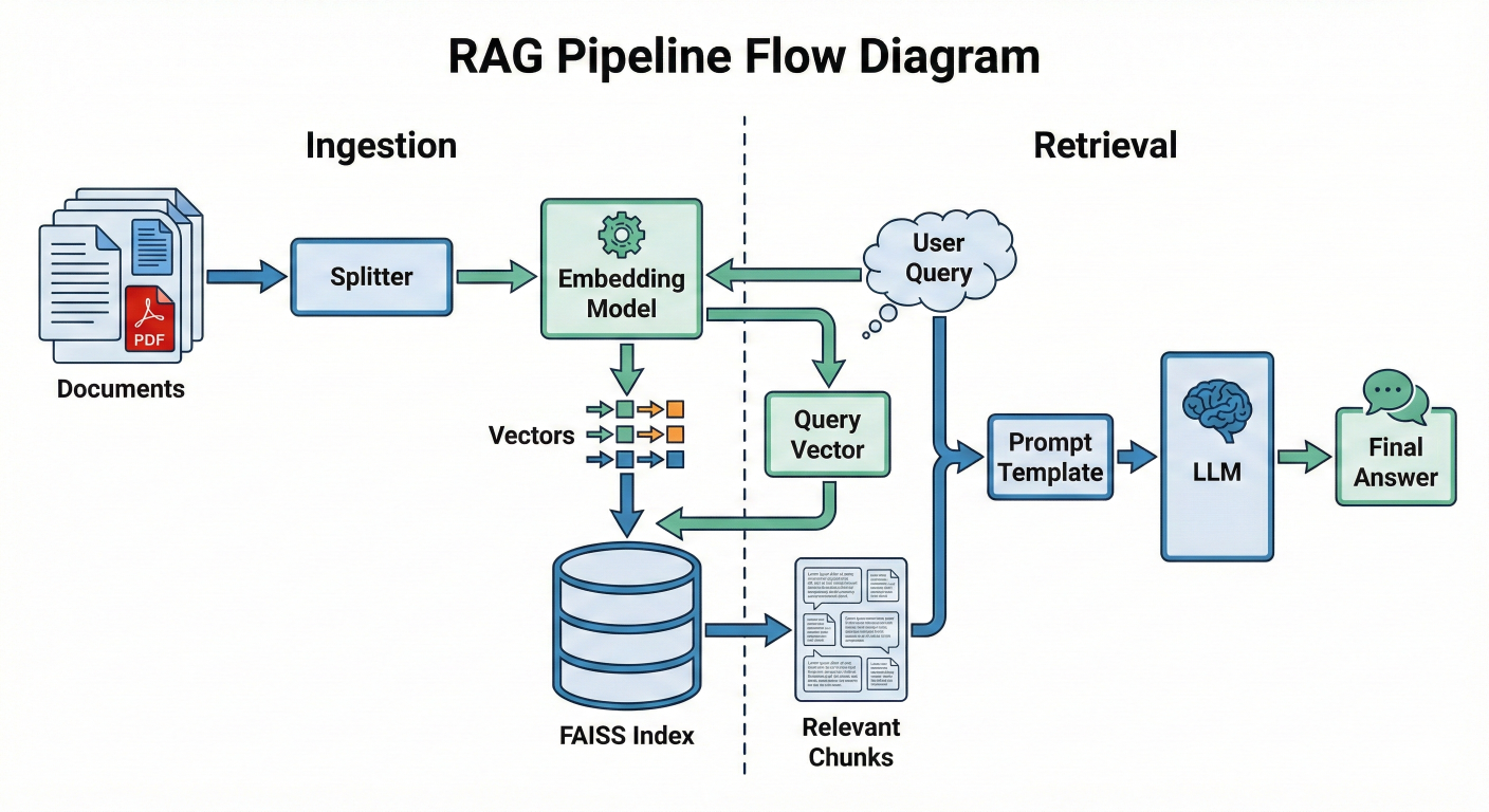
Detailed description about picture/Architecture/Diagram: A flow diagram showing the RAG pipeline. On the left (Ingestion), documents flow into a Splitter, then an Embedding Model, resulting in Vectors that go into the FAISS Index. On the right (Retrieval), a User Query flows into the same Embedding Model, producing a Query Vector. This Query Vector hits the FAISS Index, which outputs "Relevant Chunks". These chunks join the User Query in a Prompt Template, which feeds into the LLM, producing the Final Answer.
You might ask: "Why do I need a special library? Can't I just use NumPy to calculate the distance between my query and my database?"
If you have 1,000 documents, yes, you can. You can loop through them, calculate the distance, and pick the smallest one. This is called $O(N)$ complexity—linear time.
But Generative AI applications rarely stay small. When you scale to 1 million, 10 million, or 1 billion vectors, a linear scan becomes impossibly slow. Even with optimized matrix operations, comparing a 1536-dimensional vector against 1 billion vectors takes too long for a user waiting for a chatbot response.
FAISS solves this by providing algorithms that are sub-linear. Through techniques like clustering (IVF), graph traversal (HNSW), and quantization (PQ), FAISS can find the nearest neighbors in a dataset of billions without checking every single item. It trades a tiny, often imperceptible amount of accuracy (recall) for massive gains in speed.
FAISS is a library for similarity search of dense vectors. It does not understand text, images, or audio files. It only understands lists of numbers. Therefore, the quality of your FAISS implementation is entirely dependent on the quality and nature of your vectors.
A dense vector is a list of floating-point numbers that represents the semantic meaning of a piece of data. In the context of AI, we map "meaning" to "position" in a high-dimensional space.
Imagine a 2-dimensional graph with an X and Y axis. You can plot the word "King" at coordinates You can plot "Queen" at. They are close together. You plot "Apple" at ``. It is far away.
Now, expand that concept to 1,536 dimensions (the size of OpenAI's standard embeddings) or 384 dimensions (the size of many Hugging Face models). We cannot visualize 1,536 dimensions, but the math works exactly the same. Concepts that are semantically similar are located physically close to each other in this multi-dimensional hyper-space.
Key Vector Properties for FAISS
To use FAISS effectively, you must understand three properties of your vectors:
1. Dimensionality (d)
Every vector in a FAISS index must have the exact same length (dimension).
text-embedding-3-small: 1536 dimensions.text-embedding-3-large: 3072 dimensions.2. Data Type (float32)
This is a common trap for Python developers. Python's standard float is actually a double-precision float (64-bit). NumPy often defaults to float64. FAISS expects float32 by default. If you feed float64 data to FAISS, you will often see a TypeError complaining about the descriptor or input type. You must explicitly cast your data using numpy.astype('float32') before interaction with the library.
3. Normalization
Depending on the distance metric you choose (more on this in the next section), the length (magnitude) of the vector might matter. For most semantic search tasks, we only care about the direction of the vector, not its length. Therefore, vectors are often "normalized" to have a length of 1 (Unit Vectors). This ensures that the math of "Inner Product" acts exactly like "Cosine Similarity".
How does FAISS know that "Cat" is closer to "Kitten" than "Car"? It calculates the distance between their vector representations. The choice of distance metric is the single most important configuration decision you will make, and it depends entirely on how your embedding model was trained.
1. Euclidean Distance (L2)
This is the "ruler" distance. It measures the straight-line distance between two points in space.
Formula: d(x,y)=∑(xi−yi)2faiss.METRIC_L2IndexFlatL22. Inner Product (IP)
This is the dot product of two vectors.
faiss.METRIC_INNER_PRODUCTIndexFlatIP3. Cosine Similarity (The Industry Standard)
Cosine similarity measures the cosine of the angle between two vectors. It ignores magnitude completely and focuses only on orientation.
The Catch: FAISS does not have a METRIC_COSINE flag.If you search the FAISS documentation for "Cosine," you will find that it is missing. This confuses many beginners.The Solution:Cosine Similarity is mathematically identical to the Inner Product IF AND ONLY IF the vectors are normalized (i.e., their length is exactly 1).If ||x|| = 1$ and $||y|| = 1, then the divisor in the formula becomes 1, and Cosine(x,y)=x⋅y
.
The Solution: Cosine Similarity is mathematically identical to the Inner Product IF AND ONLY IF the vectors are normalized (i.e., their length is exactly 1). If ∣∣x∣∣=1and∣∣y∣∣=1
, then the divisor in the formula becomes 1, and Cosine(x,y)=x⋅y.
Therefore, to perform Cosine Similarity search in FAISS:
METRIC_INNER_PRODUCT) index.faiss.normalize_L2(vectors).| Metric |
Direction Sensitive? |
Magnitude Sensitive? | FAISS Implementation | Best For |
| Euclidean (L2) | Yes | Yes | IndexFlatL2 | Computer Vision, Clustering |
| Inner Product | Yes | Yes | IndexFlatIP | Recommender Systems |
| Cosine |
Yes |
No | Normalize + IndexFlatIP | RAG, Semantic Search |
This is the area where FAISS truly shines and where the complexity lies. "Index" is the term FAISS uses for the data structure that holds your vectors. There is not just one type of index; there is a "Zoo" of them, each offering a different trade-off between Accuracy (Recall), Speed (Latency), and Memory (RAM)
1. IndexFlatL2 / IndexFlatIP: The Brute Force BaselineThis is the simplest index. It stores the vectors exactly as they are.
IndexIVFFlat: The Speedster (Clustering) IVF stands for Inverted File. This index speeds up search by reducing the search scope using clustering.nprobe parameter (how many clusters to check).IndexFlat is too slow.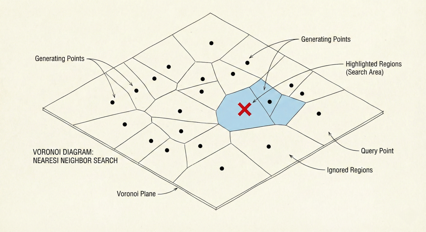
Detailed description about picture/Architecture/Diagram: A 2D visualization of Voronoi cells. Points are scattered on a plane. The plane is divided into polygonal regions. A red 'X' (query) lands in one region. The search algorithm highlights that region and perhaps one neighbor, showing that the rest of the points are ignored.
3. IndexHNSW: The Navigator (Graph-Based) HNSW stands for Hierarchical Navigable Small World. This is currently the state-of-the-art for in-memory vector search.
4. IndexPQ: The Compressor (Quantization) PQ stands for Product Quantization. This is a method for compressing vectors to reduce memory usage.
IndexIVFPQ) to enable billion-scale search on a single server.Building a FAISS index is not a "set it and forget it" process. To get production-grade performance, you need to tune specific hyperparameters. The two most critical parameters for IVF indexes are nlist and nprobe.
1. Tuning nlist (Number of Clusters)
nlist defines how many buckets (clusters) you split your data into. You set this when you create the index.
2. Tuning nprobe (Number of Probes)nprobe defines how many of those buckets you actually search for a query. This is set at search time, meaning you can change it for every query without rebuilding the index.
nprobe is your direct dial between Speed and Accuracy.nprobe = 1: Fastest possible search. You only check the single closest cluster. Risk of missing neighbors is high.nprobe = nlist: Equivalent to Brute Force. You check every cluster. Highest accuracy, slowest speed.nlist.nprobe from 1 up to 100. Measure Recall@10 and Latency for each step.nprobe that meets your accuracy requirement (e.g., 95% recall).3. GPU Acceleration
FAISS provides a highly optimized GPU implementation using CUDA.
faiss.index_cpu_to_gpu and faiss.index_gpu_to_cpu.cuVS library for even faster graph-based search (CAGRA), which can outperform HNSW on GPU.Enough theory. Let's write Python code to build a RAG-ready vector search engine. We will use SentenceTransformers to generate embeddings and FAISS to index them.
Prerequisites:
pip install faiss-cpu sentence-transformers numpy # Or 'pip install faiss-gpu' if you have an NVIDIA GPUStep 1: Generating Embeddings
First, we need to transform text into vectors. We will use the all-MiniLM-L6-v2 model, which is a great balance of speed and quality (384 dimensions).
# Usage example
import numpy as np
from sentence_transformers import SentenceTransformer

# 1. Initialize the Embedding Model
model = SentenceTransformer('all-MiniLM-L6-v2')

# 2. Our "Knowledge Base" (simulated chunks of data)
documents = []

# 3. Create Embeddings
# CRITICAL: normalize_embeddings=True allows us to use Inner Product
# for Cosine Similarity
embeddings = model.encode(
    documents,
    normalize_embeddings=True
)

# 4. Check Data Type
# FAISS requires float32. Numpy might give float64.
print(f"Original Type: {embeddings.dtype}")
embeddings = embeddings.astype('float32')
print(f"FAISS-Ready Type: {embeddings.dtype}")

# 5. Check Dimensions
d = embeddings.shape

print(f"Dimension: {d}")  # Should be 384
Step 2: Creating and Indexing with FAISS
We will start with IndexFlatIP. Since our vectors are normalized, this performs an exact Cosine Similarity search.
import faiss

# 1. Create the Index
# IndexFlatIP = Exact Search using Inner Product
index = faiss.IndexFlatIP(d)

# 2. Add Vectors to the Index
# FAISS indexes usually do not store the text, only the vectors.
index.add(embeddings)

# 3. Verification
print(f"Total vectors in index: {index.ntotal}")
Step 3: Searching
Now we simulate a user query.
# 1. User Query
query_text = "How do we store memory in AI?"

# 2. Vectorize the Query
# Must use the SAME model and settings as the database

query_vector = model.encode([query_text], normalize_embeddings=True)
query_vector = query_vector.astype('float32')

# 3. Search
# k = number of nearest neighbors to retrieve

k = 3
distances, indices = index.search(query_vector, k)

# 4. Display Results

print("\n--- Search Results ---")

for i in range(k):

    doc_id = indices[i]
    score = distances[i]

    print(f"Rank {i+1}:")
    print(f"   Score: {score:.4f}")
    print(f"   Text:  {documents[doc_id]}")
    print("-" * 30)
Expected Output: The search should prioritize the sentence about "FAISS" or "RAG" or "Vectors" as they are semantically closest to "memory in AI."
Step 4: Metadata Management – The Missing Piece
You will notice that FAISS returned indices (integers like 0, 5, 2), not the text itself. FAISS is purely a math engine; it is not a relational database. It does not know what your vectors represent.In a real production system, you must maintain a Mapping Layer.
index_id corresponds to list position.IndexIDMap, insert vector into FAISS with that specific Int ID.WHERE id IN (...) to get the text.IndexIDMap for Custom IDs: By default, FAISS assigns sequential IDs (0, 1, 2...). If your database IDs are non-sequential (e.g., 105, 109, 204), you need IndexIDMap.# Create the base index base_index = faiss.IndexFlatIP(d) # Wrap it in IDMap index_with_ids = faiss.IndexIDMap(base_index) # Custom IDs (must be integers, typically 64-bit) custom_ids = np.array().astype('int64') # Add with IDs index_with_ids.add_with_ids( embeddings, custom_ids ) # Search now returns your custom IDs D, I = index_with_ids.search( query_vector, k ) print( f"Retrieved Custom IDs: {I}" )
Since FAISS indexes reside in RAM, if your Python script terminates or the server restarts, your index (and all that "memory") is lost. You must implement persistence.
FAISS provides native read/write functions.
# Save to disk
faiss.write_index(index_with_ids, "my_rag_index.faiss")

# Load from disk
loaded_index = faiss.read_index("my_rag_index.faiss")
Warning on Pickling: Do not use Python's standard pickle module for FAISS indexes, especially if they are GPU-backed or contain complex wrappers. The internal C++ pointers may not serialize correctly. Always use faiss.write_index.
In the Generative AI boom, a new category of infrastructure has emerged: The Vector Database. Tools like Pinecone, Milvus, Weaviate, and ChromaDB are extremely popular.
A common question from developers is: "Why should I use FAISS directly when Pinecone exists?"
The answer lies in the distinction between a Library (FAISS) and a System (Vector DB).
| Feature |
FAISS (Library) | Managed Vector DBs (Pinecone, Weaviate, etc.) |
| Nature | Low-level C++ Library with Python bindings. | Full Database Management System (DBMS). |
| Hosting | Self-hosted. You run it in your RAM. | SaaS (Cloud) or Self-hosted via Docker. |
| Scaling | Vertical (get a bigger server). Horizontal scaling requires you to write custom sharding code. | Horizontal scaling is usually built-in and managed. |
| CRUD | Very difficult. Deleting specific vectors is slow/complex in many index types. Updating usually means Delete + Add. | Full CRUD support (Create, Read, Update, Delete) is standard. |
| Metadata | None. You must manage metadata separately. | Native metadata filtering (e.g., WHERE author='John'). |
| Cost | Free (Open Source). You pay only for compute. | Tiered pricing. Can get expensive at scale. |
| Under the Hood |
It is the engine. | Often uses FAISS or HNSWlib internally. |
When to use FAISS?
When to use a Vector DB?
Even experienced engineers trip over FAISS quirks. Here are the most common issues you will encounter and how to solve them.
1. The "Float64" / "Double" Error
TypeError: descriptor 'add' requires a 'faiss.Index' object but received a 'numpy.ndarray' or assertion failures regarding data types.float64 arrays by default. FAISS is strictly float32.vectors.astype('float32').IndexFlat to IndexIVFPQ. PQ compresses vectors significantly (e.g., from 4096 bytes to 32 bytes)..add() at once. Add them in batches of 50,000.Assertion 'd == this->d' failed.d.faiss-gpu alongside PyTorch (e.g., running the embedding model on GPU), you might fight for VRAM.index_gpu_to_cpu) when not actively searching to free up VRAM for the LLM.FAISS is not just a tool; it is a foundational component of the modern AI stack. By enabling efficient similarity search, it decouples the reasoning capability of an LLM from the knowledge storage of a database. This separation of concerns is what makes systems like RAG scalable, updatable, and hallucination-resistant.
As we look to the future, we see FAISS evolving. We are seeing tighter integration with NPUs (Neural Processing Units), support for binary quantization (1-bit vectors) to further reduce memory, and hybrid search capabilities that blend keyword and vector scores.
For the Generative AI developer, the path is clear: mastering the model is only half the battle. Mastering the retrieval—the memory—is where the competitive advantage lies. And in the world of retrieval, FAISS remains the gold standard.
IVFFlat index.nlist and nprobe on that dataset to see the speed vs. accuracy trade-off in real-time.
{{AUTHOR}}
 Launch your Graphy